Build and train neural networks from scratch

Overview

A lot of theoretical knowledge have been told before, now it's time to start the practice. Let's try to build a neural network from scratch and train it to string the whole process together.

In order to be more intuitive and easier to understand, we follow the following principles:

1. Do not use third-party libraries to make the logic simpler;
2. No performance optimization: avoid introducing additional concepts and techniques, increasing complexity;

Dataset

First, we need a dataset. To facilitate visualization, we use a binary function as the objective function, and then generate the dataset by sampling on it.

Note: In actual engineering projects, the objective function is unknown, but we can sample on it.

Objective function

$$o(x, y) = \begin{cases} 1 & x^2 + y^2 < 1 \\ 0 & \text{otherwise}\end{cases}$$

Code show as below:

def o(x, y):
    return 1.0 if x*x + y*y < 1 else 0.0

Generate dataset

sample_density = 10
xs = [
    [-2.0 + 4 * x/sample_density, -2.0 + 4 * y/sample_density]
    for x in range(sample_density+1)
    for y in range(sample_density+1)
]
dataset = [
    (x, y, o(x, y))
    for x, y in xs
]

The dataset generated is: [[-2.0, -2.0, 0.0], [-2.0, -1.6, 0.0], ...]

Construct a neural network

Activation function

import math

def sigmoid(x):
    return 1 / (1 + math.exp(-x))

Neuron

from random import seed, random

seed(0)

class Neuron:
    def __init__(self, num_inputs):
        self.weights = [random()-0.5 for _ in range(num_inputs)]
        self.bias = 0.0

    def forward(self, inputs):
        # z = wx + b
        z = sum([
            i * w
            for i, w in zip(inputs, self.weights)
        ]) + self.bias
        return sigmoid(z)

The neuron expression is:

$$\text{sigmoid}(\mathbf w \mathbf x + b)$$

• $\mathbf w$: vector, corresponding to the weights array in the code
• $b$: corresponds to the bias in the code

Note: The parameters in the neuron are initialized randomly. However, in order to ensure reproducible experiments, a random seed is set(seed(0))

Neural Networks

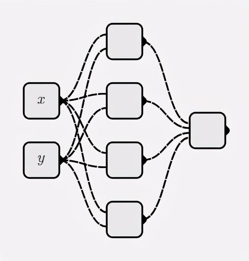
class MyNet:
    def __init__(self, num_inputs, hidden_shapes):
        layer_shapes = hidden_shapes + [1]
        input_shapes = [num_inputs] + hidden_shapes
        self.layers = [
            [
                Neuron(pre_layer_size)
                for _ in range(layer_size)
            ]
            for layer_size, pre_layer_size in zip(layer_shapes, input_shapes)
        ]

    def forward(self, inputs):
        for layer in self.layers:
            inputs = [
                neuron.forward(inputs)
                for neuron in layer
            ]
        # return the output of the last neuron
        return inputs[0]

Construct a neural network as follows:

net = MyNet(2, [4])

At this point, we have got a neural network(net), which can call its neural network function:

print(net.forward([0, 0]))

Get the function value 0.55..., the neural network at this time is an untrained network.

Train the neural network

Loss function

First define a loss function:

def square_loss(predict, target):
    return (predict-target)**2

Calculate the gradient

The calculation of the gradient is complicated, especially for deep neural networks. Back Propagation Algorithm is an algorithm specifically designed to calculate the gradient of a neural network.

Due to its complexity, it will not be described here. Those interested can refer to the following detailed code. Moreover, the current deep learning framework has the function of automatically calculating the gradient.

Define the derivative function:

def sigmoid_derivative(x):
    _output = sigmoid(x)
    return _output * (1 - _output)

def square_loss_derivative(predict, target):
    return 2 * (predict-target)

Find the partial derivative (part of the data is cached in the forward function to facilitate the derivative):

class Neuron:
    ...

    def forward(self, inputs):
        self.inputs_cache = inputs

        # z = wx + b
        self.z_cache = sum([
            i * w
            for i, w in zip(inputs, self.weights)
        ]) + self.bias
        return sigmoid(self.z_cache)

    def zero_grad(self):
        self.d_weights = [0.0 for w in self.weights]
        self.d_bias = 0.0

    def backward(self, d_a):
        d_loss_z = d_a * sigmoid_derivative(self.z_cache)
        self.d_bias += d_loss_z
        for i in range(len(self.inputs_cache)):
            self.d_weights[i] += d_loss_z * self.inputs_cache[i]
        return [d_loss_z * w for w in self.weights]


class MyNet:
    ...

    def zero_grad(self):
        for layer in self.layers:
            for neuron in layer:
                neuron.zero_grad()

    def backward(self, d_loss):
        d_as = [d_loss]
        for layer in reversed(self.layers):
            da_list = [
                neuron.backward(d_a)
                for neuron, d_a in zip(layer, d_as)
            ]
            d_as = [sum(da) for da in zip(*da_list)]

• Partial derivatives are stored in d_weights and d_bias respectively
• The zero_grad function is used to clear the gradient, including each partial derivative
• The backward function is used to calculate the partial derivative and store its value cumulatively

Update parameters

Use gradient descent method to update parameters:

class Neuron:
    ...

    def update_params(self, learning_rate):
        self.bias -= learning_rate * self.d_bias
        for i in range(len(self.weights)):
            self.weights[i] -= learning_rate * self.d_weights[i]


class MyNet:
    ...

    def update_params(self, learning_rate):
        for layer in self.layers:
            for neuron in layer:
                neuron.update_params(learning_rate)

Perform training

def one_step(learning_rate):
    net.zero_grad()

    loss = 0.0
    num_samples = len(dataset)
    for x, y, z in dataset:
        predict = net.forward([x, y])
        loss += square_loss(predict, z)

        net.backward(square_loss_derivative(predict, z) / num_samples)

    net.update_params(learning_rate)
    return loss / num_samples


def train(epoch, learning_rate):
    for i in range(epoch):
        loss = one_step(learning_rate)
        if i == 0 or (i+1) % 100 == 0:
            print(f"{i+1} {loss:.4f}")

Training 2000 steps:

train(2000, learning_rate=10)

Note: A relatively large learning rate is used here, which is related to the project situation. The learning rate in actual projects is usually very small

$\text{log y}$

Inference

After training, the model can be used for inference:

def inference(x, y):
    return net.forward([x, y])

print(inference(1, 2))

Please refer to the complete code: nn_from_scratch.py

Summary

The steps of this practice are as follows:

1. Construct a virtual objective function: $o(x, y)$;
2. Sampling on $o(x, y)$ to get the dataset, that is, the dataset function: $d(x, y)$
3. Constructed a fully connected neural network with a hidden layer, that is, neural network function: $f(x, y)$
4. Use the gradient descent method to train the neural network so that $f(x, y)$ approximates $d(x, y)$

The most complicated part is to find the gradient, which uses the back-propagation algorithm. In actual projects, using mainstream deep learning frameworks for development can save the code for gradients and lower the threshold.

In the laboratory's 3D classification experiments, the second dataset is very similar to the one in this practice, so you can go in and operate it.